GSP774

Overview

In this lab you will explore the financial transactions data for fraud analysis, apply feature engineering and machine learning techniques to detect fraudulent activities using BigQuery ML.

Public financial transactions data will be used. The data contains the following columns:

• Type of the transaction
• Amount transferred
• Account id of origin and destination
• New and old balances
• Relative time of transaction (number of hours from the start of the 30-day period)
• isfraud flag

The target column isfraud includes the labels for the fraudulent transactions. Using these labels you will train supervised models for fraud detection and apply unsupervised models to detect anomalies.

The data for this lab is from the Kaggle site. If you do not have a Kaggle account, it's free to create one.

What you'll learn:

• Load data into BigQuery and explore.
• Create new features in BigQuery.
• Build an unsupervised model for anomaly detection.
• Build supervised models (with logistic regression and boosted tree) for fraud detection.
• Evaluate and compare the models and select the champion.
• Use the selected model to predict the likelihood of fraud on a test data.

In this lab, you will use the BigQuery interface for feature engineering, model development, evaluation and prediction.

Participants that prefer Notebooks as the model development interface may choose to build models in AI Platform Notebooks instead of BigQuery ML. Then at the end of the lab, you can also complete the optional section. You can import open source libraries and create custom models or you can call BigQuery ML models within Notebooks using BigQuery magic commands.

If you want to train models in an automated way without any coding, you can use Google Cloud AutoML which builds models using state-of-the-art algorithms. The training process for AutoML would take almost 2 hours, that's why it is recommended to initiate it at the beginning of the lab, as soon as the data is prepared, so that you can see the results at the end. Check for the "Attention" phrase at the end of the data preparation step.

Setup and requirements

Before you click the Start Lab button

Read these instructions. Labs are timed and you cannot pause them. The timer, which starts when you click Start Lab, shows how long Google Cloud resources will be made available to you.

This hands-on lab lets you do the lab activities yourself in a real cloud environment, not in a simulation or demo environment. It does so by giving you new, temporary credentials that you use to sign in and access Google Cloud for the duration of the lab.

To complete this lab, you need:

• Access to a standard internet browser (Chrome browser recommended).

Note: Use an Incognito or private browser window to run this lab. This prevents any conflicts between your personal account and the Student account, which may cause extra charges incurred to your personal account.

• Time to complete the lab---remember, once you start, you cannot pause a lab.

Note: If you already have your own personal Google Cloud account or project, do not use it for this lab to avoid extra charges to your account.

How to start your lab and sign in to the Google Cloud console

1. Click the Start Lab button. If you need to pay for the lab, a pop-up opens for you to select your payment method. On the left is the Lab Details panel with the following:

   • The Open Google Cloud console button
   • Time remaining
   • The temporary credentials that you must use for this lab
   • Other information, if needed, to step through this lab

2. Click Open Google Cloud console (or right-click and select Open Link in Incognito Window if you are running the Chrome browser).

   The lab spins up resources, and then opens another tab that shows the Sign in page.

   Tip: Arrange the tabs in separate windows, side-by-side.

   Note: If you see the Choose an account dialog, click Use Another Account.

3. If necessary, copy the Username below and paste it into the Sign in dialog.

   {{{user_0.username | "Username"}}}

   You can also find the Username in the Lab Details panel.

4. Click Next.

5. Copy the Password below and paste it into the Welcome dialog.

   {{{user_0.password | "Password"}}}

   You can also find the Password in the Lab Details panel.

6. Click Next.

   Important: You must use the credentials the lab provides you. Do not use your Google Cloud account credentials. Note: Using your own Google Cloud account for this lab may incur extra charges.

7. Click through the subsequent pages:

   • Accept the terms and conditions.
   • Do not add recovery options or two-factor authentication (because this is a temporary account).
   • Do not sign up for free trials.

After a few moments, the Google Cloud console opens in this tab.

Note: To view a menu with a list of Google Cloud products and services, click the Navigation menu at the top-left.

Activate Cloud Shell

Cloud Shell is a virtual machine that is loaded with development tools. It offers a persistent 5GB home directory and runs on the Google Cloud. Cloud Shell provides command-line access to your Google Cloud resources.

1. Click Activate Cloud Shell at the top of the Google Cloud console.

When you are connected, you are already authenticated, and the project is set to your Project_ID, . The output contains a line that declares the Project_ID for this session:

Your Cloud Platform project in this session is set to {{{project_0.project_id | "PROJECT_ID"}}}

gcloud is the command-line tool for Google Cloud. It comes pre-installed on Cloud Shell and supports tab-completion.

2. (Optional) You can list the active account name with this command:

gcloud auth list

3. Click Authorize.

Output:

ACTIVE: * ACCOUNT: {{{user_0.username | "ACCOUNT"}}} To set the active account, run: $ gcloud config set account `ACCOUNT`

4. (Optional) You can list the project ID with this command:

gcloud config list project

Output:

[core] project = {{{project_0.project_id | "PROJECT_ID"}}} Note: For full documentation of gcloud, in Google Cloud, refer to the gcloud CLI overview guide.

Task 1. Download the data file for the lab

1. Run the following to download the data file to your project:

gsutil cp gs://spls/gsp774/archive.zip .

2. If prompted, click Authorize.

3. Once you upload your zip file, run the unzip command:

unzip archive.zip

You will see that 1 file has been inflated.

4. In order to make it easier to refer to this file later, create an environment variable for the name of the file:

export DATA_FILE=PS_20174392719_1491204439457_log.csv

5. Run the following to find the Project ID for your lab, then copy the Project ID:

gcloud config list project

6. Create an environment variable for the Project ID and replace <project_id> with the copied Project ID:

export PROJECT_ID=<project_id>

7. Run the following to create a BigQuery Dataset to store tables and models for this lab called finance in Cloud Shell:

bq mk --dataset $PROJECT_ID:finance

Successful execution of the above command will result with the output:

Dataset `$PROJECT_ID:finance` successfully created.

Click Check my progress to verify the objective. Create a dataset

Task 2. Copy dataset to Cloud Storage

1. Run the following to create a Cloud Storage bucket using your unique Project ID as its name:

gsutil mb gs://$PROJECT_ID

2. Copy your csv file into your newly created bucket:

gsutil cp $DATA_FILE gs://$PROJECT_ID

Task 3. Load data to BigQuery tables

To load your data into BigQuery you can either use the BigQuery user interface or the command terminal in Cloud Shell. Choose one of the options below to load your data.

Option 1: Command line

• Load data from into the table finance.fraud_data by executing the following command:

bq load --autodetect --source_format=CSV --max_bad_records=100000 finance.fraud_data gs://$PROJECT_ID/$DATA_FILE

The option --autodetect will read the schema of the table (the variable names, types, etc.) automatically.

Option 2: BigQuery user interface

You can load data from your Cloud Storage bucket by opening BigQuery in the Cloud Console.

1. Click on Expand node next to your Project ID in the Explorer section.
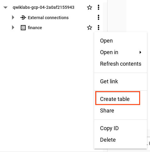
2. Click View actions next to the finance dataset and then click Create Table.

3. In the Create table pop-up window, set Source as Google Cloud Storage and select the raw csv file in your Cloud Storage bucket.

4. Enter table name as fraud_data and select the Auto detect option under Schema so that the variable names will be read from the first line of the raw file automatically.

5. Click Create table.

The loading process can take one or two minutes.

6. Once completed, in the Explorer panel view in BigQuery, click on the finance dataset and find the table fraud_data to view the metadata and preview the table data.

Click Check my progress to verify the objective. Load Data to BigQuery Tables

Task 4. Explore and investigate the data with BigQuery

If you haven't opened BigQuery in the Cloud Console, yet, do it now.

1. Click on Navigation menu > BigQuery.

Next you'll start exploring the data in order to understand it better and prepare it for machine learning models.

2. Add the following queries to the query EDITOR, then click RUN, then explore the data.

3. Click COMPOSE NEW QUERY to start the next query. This will let you compare results easily when you're done.

• What is the number of fraudulent transactions for each transaction type?

SELECT type, isFraud, count(*) as cnt FROM `finance.fraud_data` GROUP BY isFraud, type ORDER BY type

Look in the isFraud column for 1 = yes.

• Run the following to see the proportion of fraudulent activities for the transaction types of TRANSFER and CASH_OUT (it gives the counts of isFraud):

SELECT isFraud, count(*) as cnt FROM `finance.fraud_data` WHERE type in ("CASH_OUT", "TRANSFER") GROUP BY isFraud

• Run the following to see the top 10 maximum amounts of transactions:

SELECT * FROM `finance.fraud_data` ORDER BY amount desc LIMIT 10

PAUSE and REFLECT:

• Have you noticed any interesting balance amounts in the transactions? How can you make a transaction when the balance in the origin account is zero? Why does the new balance in the destination account stay zero after the money transfer? We will flag these cases and add them as new features in the next step.
• Do you think the data is imbalanced? Yes, the proportion of fraudulent transactions is much less than 1%? When you divide the isfraud number by the total number of observations you get the proportion of fraudulent transactions.

In the next section, you will see how to handle these questions and improve the data for machine learning models.

Click Check my progress to verify the objective. Explore and Investigate the Data with BigQuery

Task 5. Prepare your data

You can improve the modelling data by adding new features, filtering unnecessary transaction types, and increasing the proportion of the target variable isFraud by applying undersampling.

Based on your findings from the analysis phase, you only need to analyse the transaction types "TRANSFER" and "CASH_OUT" and filter the rest. You can also compute new variables from the existing amount values.

The dataset contains an extremely unbalanced target for fraud (fraud rate in the raw data = 0.0013%). Having rare events is common for fraud. In order to make the pattern of fraudulent behaviour more obvious for the machine learning algorithms, and also make it easy to interpret the results, stratify the data and increase the proportion of the fraudulent flags.

1. In the next step, compose a new query add the following code to add new features to the data, filter unnecessary transaction types and select a subset of the non-fraud transactions with undersampling:

CREATE OR REPLACE TABLE finance.fraud_data_sample AS SELECT type, amount, nameOrig, nameDest, oldbalanceOrg as oldbalanceOrig, #standardize the naming. newbalanceOrig, oldbalanceDest, newbalanceDest, # add new features: if(oldbalanceOrg = 0.0, 1, 0) as origzeroFlag, if(newbalanceDest = 0.0, 1, 0) as destzeroFlag, round((newbalanceDest-oldbalanceDest-amount)) as amountError, generate_uuid() as id, #create a unique id for each transaction. isFraud FROM finance.fraud_data WHERE # filter unnecessary transaction types: type in("CASH_OUT","TRANSFER") AND # undersample: (isFraud = 1 or (RAND()< 10/100)) # select 10% of the non-fraud cases

2. Run the query.

3. Create a TEST data table by selecting a random sample of 20%:

CREATE OR REPLACE TABLE finance.fraud_data_test AS SELECT * FROM finance.fraud_data_sample where RAND() < 20/100

4. Run the query.

This data will be kept separate and not be included in training. You will use it for scoring the model at the final stage.

BigQuery ML and AutoML will automatically partition the model data as TRAIN and VALIDATE while using the machine learning algorithms in order to test the error rate on both the training and validation data and avoid overfitting.

5. Run the following to create sample data:

CREATE OR REPLACE TABLE finance.fraud_data_model AS SELECT * FROM finance.fraud_data_sample EXCEPT distinct select * from finance.fraud_data_test

The sample data that you created for modelling contains approximately 228k rows of banking transactions.

You can also manually partition your data set as TRAIN/VALIDATE and TEST, especially when you want to compare models from different environments such as AutoML or AI Platform and have consistency.

PAUSE and REFLECT:

• How would you approach this problem of having no labelled fraud events in the data? If there are no labelled transactions, then you can use unsupervised modeling techniques to analyse anomalies in the data such as k-means clustering. In the next section you will try this method yourself.

Click Check my progress to verify the objective. Prepare Your Data

Task 6. Train an unsupervised model to detect dnomalies

Unsupervised methods are commonly used in fraud detection to explore the abnormal behaviour in the data. It also helps when there are no labels for fraud or the event rate is very low and the number of occurrences does not allow you to build a supervised model.

In this section, you will use k-means clustering algorithm to create segments of transactions, analyse each segment and detect the ones with anomalies.

1. Compose a new query and run the code below in BigQuery with CREATE or REPLACE MODEL and set the model_type as kmeans:

CREATE OR REPLACE MODEL finance.model_unsupervised OPTIONS(model_type='kmeans', num_clusters=5) AS SELECT amount, oldbalanceOrig, newbalanceOrig, oldbalanceDest, newbalanceDest, type, origzeroFlag, destzeroFlag, amountError FROM `finance.fraud_data_model`

This will create a k-means model called model_unsupervised with 5 clusters using the selected variables from fraud_data_model.

Note: It will take a few minutes for the model to finish training.

Once the model finishes training you will see it appear under Finance > Models.

2. Click on model_unsupervised, then click on the EVALUATION tab.

The k-means algorithm creates an output variable called centroid_id. Each transaction is assigned to a centroid_id. The transactions that are similar/closer to each other are assigned to the same cluster by the algorithm.

The Davies-Bouldin index shows an indication of how homogeneous the clusters are. The lower the value is, the more distant the clusters are from each other which is the desired outcome.

The numeric features are displayed with bar charts for each centroid (cluster) in the Evaluation tab. The numbers next to the bars show the average value of the variables within each cluster. As a best practice, the input variables can be standardized or grouped into buckets in order to avoid the impact of large numbers or outliers in the distance calculations for clustering. For the sake of simplicity, this lab uses the original variables in this exercise.

The categorical variables that are used as input are displayed separately. You can see the distribution of TRANSFER and CASH_OUT transactions in each segment below.

The charts might look different for your model, focus on the smaller segments and try to interpret the distributions.

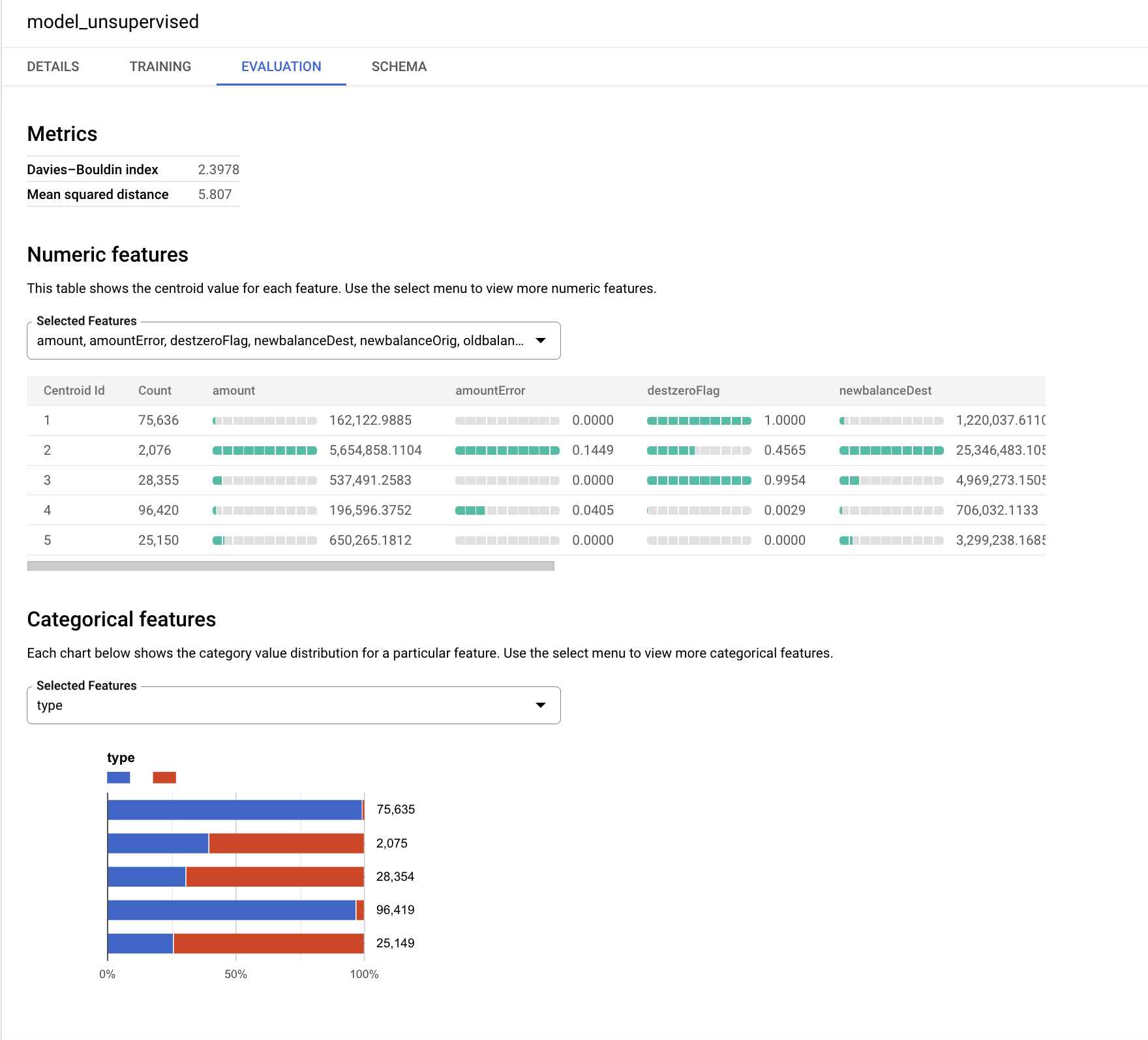
The target variable isFraud hasn't been used in this unsupervised model. In this exercise, it is preferred to save that variable for profiling and use it to explore the distribution of fraudulent activities within each cluster.

3. Score the test data (fraud_data_test) using this model and see the number of fraud events in each centroid_id. The clustering algorithms create homogeneous groups of observations. In this query, ML.PREDICT will call the model and generate the centroid_id for each transaction in the test data.

4. Run the following code in new query:

SELECT centroid_id, sum(isfraud) as fraud_cnt, count(*) total_cnt FROM ML.PREDICT(MODEL `finance.model_unsupervised`, ( SELECT * FROM `finance.fraud_data_test`)) group by centroid_id order by centroid_id

PAUSE and REFLECT:

• Which cluster do you think is the most interesting one? That would be the small clusters with high error amounts.

Click Check my progress to verify the objective. Train an Unsupervised Model to Detect Anomalies

Task 7. Train a supervised machine learning model

Now you are ready to start building supervised models using BigQuery ML to predict the likelihood of having fraudulent transactions. Start with a simple model - use BigQuery ML to create a binary logistic regression model for classification. This model will attempt to predict if the transaction is likely to be fraudulent or not.

For all non-numeric (categorical) variables, BigQuery ML automatically performs a one-hot encoding transformation. This transformation generates a separate feature for each unique value in the variable. In this exercise, one-hot encoding will be performed for the variable TYPE automatically by BigQuery ML.

1. To create your first supervised model, execute the following SQL statement in BigQuery:

CREATE OR REPLACE MODEL finance.model_supervised_initial OPTIONS(model_type='LOGISTIC_REG', INPUT_LABEL_COLS = ["isfraud"] ) AS SELECT type, amount, oldbalanceOrig, newbalanceOrig, oldbalanceDest, newbalanceDest, isFraud FROM finance.fraud_data_model Note: It takes a few minutes for BigQuery to create and train this logistic regression model.

You will see model_supervised_initial table added under Finance > Models when it is ready.

Once the model is created you can get the model metadata, training, and evaluation stats from BigQuery Console UI.

2. Click on model_supervised_initial in the left side panel, then click on the Details, Training, Evaluation, or Schema tab to get more information.

On the Evaluation tab, you will find various performance metrics specific to the classification model.

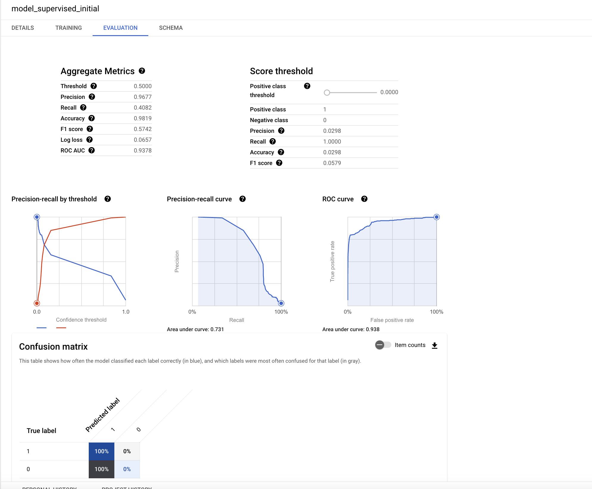
Understanding performance of the model is a key topic in machine learning. Since you performed a logistic regression for classification, the following key concepts are useful to understand:

• precision: Precision identifies the proportion of selected positive cases where the model was correct.
• recall: A metric that answers the following: Out of all the possible positive actual labels, how many did the model correctly identify?
• accuracy: Accuracy is the overall proportion of correct predictions.
• f1 score: A measure of the accuracy of the model. The f1 score is the harmonic average of the precision and recall, taking values from 0 to 1, the higher the better.
• roc, auc: The area under the ROC curve. This gives information about the discrimination capability of a binary classifier considering different thresholds, taking values between 0 and 1, the higher the better. For a moderate model, the expectation would be having a ROC value greater than 0.7.

The chart in this wikipedia page explains the concepts of precision and recall nicely.

The ROC value for this regression model is very high. You can get a better understanding of the accuracy by testing the outcomes for different probability thresholds.

Now, look at the most influential features in the model.

3. Run the following query to check feature importance:

SELECT * FROM ML.WEIGHTS(MODEL `finance.model_supervised_initial`, STRUCT(true AS standardize))

The weights are standardized to eliminate the impact of the scale of the variables using the standardize option. The larger weights are the more important ones. The sign of the weight indicates the direction, depending on the direct or inverse relationship with the target.

PAUSE and REFLECT:

• Which two variables look the most important? oldbalanceOrig and type are the most important variables.

Click Check my progress to verify the objective. Train a Supervised Machine Learning Model

Task 8. Improve your model

Now do a fun exercise - create a new model and train the two models to get better accuracy.

• Create a new gradient boost model by running the following:

CREATE OR REPLACE MODEL finance.model_supervised_boosted_tree OPTIONS(model_type='BOOSTED_TREE_CLASSIFIER', INPUT_LABEL_COLS = ["isfraud"] ) AS SELECT type, amount, oldbalanceOrig, newbalanceOrig, oldbalanceDest, newbalanceDest, isFraud FROM finance.fraud_data_model Note: It will take a few minutes for the model to finish training.

Next, you will compare the 2 models you created and choose the best one.

Task 9. Evaluate your supervised machine learning models

Improve the existing logistic regression model by adding new variables.

After creating the model, you can evaluate the performance of the classifier using ML.EVALUATE function. The ML.EVALUATE function evaluates the outcome or predicted values against actual data.

• Run the following queries in order to append the results from the two models in a single table and choose the champion model to use for scoring new data.

CREATE OR REPLACE TABLE finance.table_perf AS SELECT "Initial_reg" as model_name, * FROM ML.EVALUATE(MODEL `finance.model_supervised_initial`, ( SELECT * FROM `finance.fraud_data_model` )) insert finance.table_perf SELECT "improved_reg" as model_name, * FROM ML.EVALUATE(MODEL `finance.model_supervised_boosted_tree`, ( SELECT * FROM `finance.fraud_data_model` ))

PAUSE and REFLECT:

• Which model has given the best performance? Initially you ran a regression model. You then added more variables and trained a new model using regression (the supervised model). Finally you used boosted tree as the second supervised model. The boosted tree model performs better when you compare the performance tables. Adding the new, additional features improved the model's accuracy.

Task 10. Predict fraudulent transactions on test data

The last step in machine learning is to use the champion model to predict the outcome on new datasets.

The machine learning algorithms in BQML create a nested variable called predicted_<target_name\>_probs. This variable includes the probability scores for the model decision. The decision for your model is either being fraudulent or genuine.

• Run the following query in BigQuery to see the prediction of fraudulent transactions on the test data that was created at the beginning of the lab. The WHERE statement below will bring you the transactions with the highest probability scores:

SELECT id, label as predicted, isFraud as actual FROM ML.PREDICT(MODEL `finance.model_supervised_initial`, ( SELECT * FROM `finance.fraud_data_test` ) ), unnest(predicted_isfraud_probs) as p where p.label = 1 and p.prob > 0.5

PAUSE and REFLECT:

• What is the proportion of fraudulent activities in the predicted set of transactions? Less than 3%.
• How much has the event rate increased in the predicted set of rows compared to the overall test data? More than 95%.

Click Check my progress to verify the objective. Predict Fraudulent Transactions on Test Data

Congratulations!

Next steps

• Learn more about Machine Learning from Google Developers Crash Course.

Google Cloud training and certification

...helps you make the most of Google Cloud technologies. Our classes include technical skills and best practices to help you get up to speed quickly and continue your learning journey. We offer fundamental to advanced level training, with on-demand, live, and virtual options to suit your busy schedule. Certifications help you validate and prove your skill and expertise in Google Cloud technologies.

Manual Last Updated October 12, 2023

Lab Last Tested October 12, 2023

Copyright 2024 Google LLC All rights reserved. Google and the Google logo are trademarks of Google LLC. All other company and product names may be trademarks of the respective companies with which they are associated.