GSP281

Overview

SQL (Structured Query Language) is a standard language for data operations that allows you to ask questions and get insights from structured datasets. It's commonly used in database management and allows you to perform tasks like transaction record writing into relational databases and petabyte-scale data analysis.

This lab is divided into two parts: in the first half, you will learn fundamental SQL querying keywords, which you will run in BigQuery on a public dataset that contains information on London bikeshares.

In the second half, you will learn how to export subsets of the London bikeshare dataset into CSV files, which you will then upload to Cloud SQL. From there you will learn how to use Cloud SQL to create and manage databases and tables. Towards the end, you will get hands-on practice with additional SQL keywords that manipulate and edit data.

What you'll learn

In this lab, you will learn how to:

• Read data into BigQuery.
• Execute simple queries in BigQuery to explore data.
• Export a subset of data into a CSV file and store that file in a new Cloud Storage bucket.
• Create a new Cloud SQL instance and load your exported CSV file as a new table.

Prerequisites

Very Important: Before starting this lab, log out of your personal or corporate gmail account.

This is an introductory level lab. This assumes little to no prior experience with SQL. Familiarity with Cloud Storage and Cloud Shell is recommended, but not required. This lab will teach you the basics of reading and writing queries in SQL, which you will apply by using BigQuery and Cloud SQL.

Before taking this lab, consider your proficiency in SQL. Below are more challenging labs that will let you apply your knowledge to more advanced use cases:

• Weather Data in BigQuery
• Analyzing Natality Data Using Vertex AI and BigQuery

Once you're ready, scroll down and follow the steps below to get your lab environment set up.

Setup and requirements

Before you click the Start Lab button

Read these instructions. Labs are timed and you cannot pause them. The timer, which starts when you click Start Lab, shows how long Google Cloud resources will be made available to you.

This hands-on lab lets you do the lab activities yourself in a real cloud environment, not in a simulation or demo environment. It does so by giving you new, temporary credentials that you use to sign in and access Google Cloud for the duration of the lab.

To complete this lab, you need:

• Access to a standard internet browser (Chrome browser recommended).

Note: Use an Incognito or private browser window to run this lab. This prevents any conflicts between your personal account and the Student account, which may cause extra charges incurred to your personal account.

• Time to complete the lab---remember, once you start, you cannot pause a lab.

Note: If you already have your own personal Google Cloud account or project, do not use it for this lab to avoid extra charges to your account.

How to start your lab and sign in to the Google Cloud console

1. Click the Start Lab button. If you need to pay for the lab, a pop-up opens for you to select your payment method. On the left is the Lab Details panel with the following:

   • The Open Google Cloud console button
   • Time remaining
   • The temporary credentials that you must use for this lab
   • Other information, if needed, to step through this lab

2. Click Open Google Cloud console (or right-click and select Open Link in Incognito Window if you are running the Chrome browser).

   The lab spins up resources, and then opens another tab that shows the Sign in page.

   Tip: Arrange the tabs in separate windows, side-by-side.

   Note: If you see the Choose an account dialog, click Use Another Account.

3. If necessary, copy the Username below and paste it into the Sign in dialog.

   {{{user_0.username | "Username"}}}

   You can also find the Username in the Lab Details panel.

4. Click Next.

5. Copy the Password below and paste it into the Welcome dialog.

   {{{user_0.password | "Password"}}}

   You can also find the Password in the Lab Details panel.

6. Click Next.

   Important: You must use the credentials the lab provides you. Do not use your Google Cloud account credentials. Note: Using your own Google Cloud account for this lab may incur extra charges.

7. Click through the subsequent pages:

   • Accept the terms and conditions.
   • Do not add recovery options or two-factor authentication (because this is a temporary account).
   • Do not sign up for free trials.

After a few moments, the Google Cloud console opens in this tab.

Note: To view a menu with a list of Google Cloud products and services, click the Navigation menu at the top-left.

Task 1. The basics of SQL

Databases and tables

As mentioned earlier, SQL allows you to get information from "structured datasets". Structured datasets have clear rules and formatting and often times are organized into tables, or data that's formatted in rows and columns.

An example of unstructured data would be an image file. Unstructured data is inoperable with SQL and cannot be stored in BigQuery datasets or tables (at least natively.) To work with image data (for instance), you would use a service like Cloud Vision, perhaps through its API directly.

The following is an example of a structured dataset—a simple table:

User	Price	Shipped
Sean	$35	Yes
Rocky	$50	No

If you've had experience with Google Sheets, then the above should look quite similar. The table has columns for User, Price, and Shipped and two rows that are composed of filled in column values.

A Database is essentially a collection of one or more tables. SQL is a structured database management tool, but quite often (and in this lab) you will be running queries on one or a few tables joined together—not on whole databases.

SELECT and FROM

SQL is phonetic by nature and before running a query, it's always helpful to first figure out what question you want to ask your data (unless you're just exploring for fun.)

SQL has predefined keywords which you use to translate your question into the pseudo-english SQL syntax so you can get the database engine to return the answer you want.

The most essential keywords are SELECT and FROM:

• Use SELECT to specify what fields you want to pull from your dataset.
• Use FROM to specify what table or tables you want to pull our data from.

An example may help understanding. Assume that you have the following table example_table, which has columns USER, PRICE, and SHIPPED:

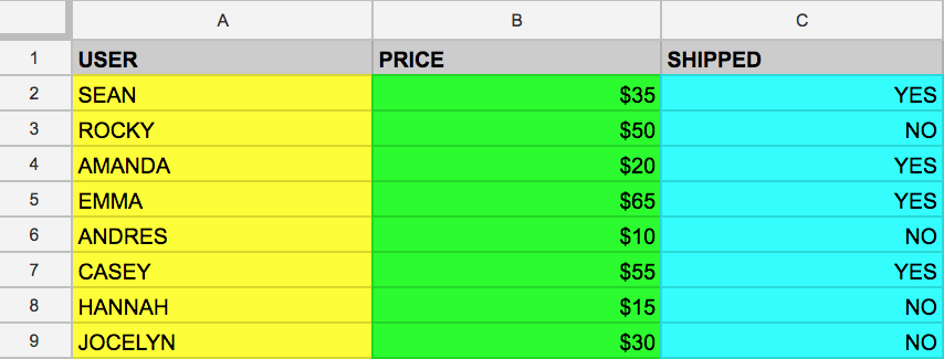
And say that you want to just pull the data that's found in the USER column. You can do this by running the following query that uses SELECT and FROM:

SELECT USER FROM example_table

If you executed the above command, you would select all the names from the USER column that are found in example_table.

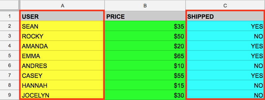
You can also select multiple columns with the SQL SELECT keyword. Say that you want to pull the data that's found in the USER and SHIPPED columns. To do this, modify the previous query by adding another column value to our SELECT query (making sure it's separated by a comma!):

SELECT USER, SHIPPED FROM example_table

Running the above retrieves the USER and the SHIPPED data from memory:

And just like that you've covered two fundamental SQL keywords! Now to make things a bit more interesting.

WHERE

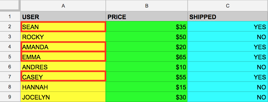
The WHERE keyword is another SQL command that filters tables for specific column values. Say that you want to pull the names from example_table whose packages were shipped. You can supplement the query with a WHERE, like the following:

SELECT USER FROM example_table WHERE SHIPPED='YES'

Running the above returns all USERs whose packages have been SHIPPED from memory:

Now that you have a baseline understanding of SQL's core keywords, apply what you've learned by running these types of queries in the BigQuery console.

Test your understanding

The following are some multiple choice questions to reinforce your understanding of the concepts covered so far. Answer them to the best of your abilities.

Task 2. Exploring the BigQuery console

The BigQuery paradigm

BigQuery is a fully-managed petabyte-scale data warehouse that runs on the Google Cloud. Data analysts and data scientists can quickly query and filter large datasets, aggregate results, and perform complex operations without having to worry about setting up and managing servers. It comes in the form of a command line tool (pre installed in cloudshell) or a web console—both ready for managing and querying data housed in Google Cloud projects.

In this lab, you use the web console to run SQL queries.

Open the BigQuery console

1. In the Google Cloud Console, select Navigation menu > BigQuery.

The Welcome to BigQuery in the Cloud Console message box opens. This message box provides a link to the quickstart guide and the release notes.

2. Click Done.

The BigQuery console opens.

Take a moment to note some important features of the UI. The right-hand side of the console houses the query "Editor". This is where you write and run SQL commands like the examples covered earlier. Below that is "Query history", which is a list of queries you ran previously.

The left pane of the console is the Navigation menu. Apart from the self-explanatory query history, saved queries, and job history, there is the Explorer tab.

The highest level of resources in the Explorer tab contain Google Cloud projects, which are just like the temporary Google Cloud projects you sign into and use with each Google Cloud Skills Boost lab. As you can see in your console and in the last screenshot, you only have your project housed in the Explorer tab. If you try clicking on the arrow next to the project name, nothing will show up.

This is because your project contains no datasets or tables, you have nothing that can be queried. Earlier you learned datasets contain tables. When you add data to your project, note that in BigQuery, projects contain datasets, and datasets contain tables. Now that you better understand the project > dataset > table paradigm and the intricacies of the console, you can load up some queryable data.

Uploading queryable data

In this section you pull in some public data into your project so you can practice running SQL commands in BigQuery.

1. Click on + ADD.

2. Choose Star a project by name.

3. Enter project name as bigquery-public-data.

4. Click STAR.

It's important to note that you are still working out of your lab project in this new tab. All you did was pull a publicly accessible project that contains datasets and tables into BigQuery for analysis — you didn't switch over to that project. All of your jobs and services are still tied to your Google Cloud Skills Boost account. You can see this for yourself by inspecting the project field near the top of the console:

5. You now have access to the following data:

• Google Cloud Project → bigquery-public-data
• Dataset → london_bicycles

6. Click on the london bicycles dataset to reveal the associated tables

• Table → cycle_hire
• Table → cycle_stations

In this lab you will use the data from cycle_hire. Open the cycle_hire table, then click the Preview tab. Your page should resemble the following:

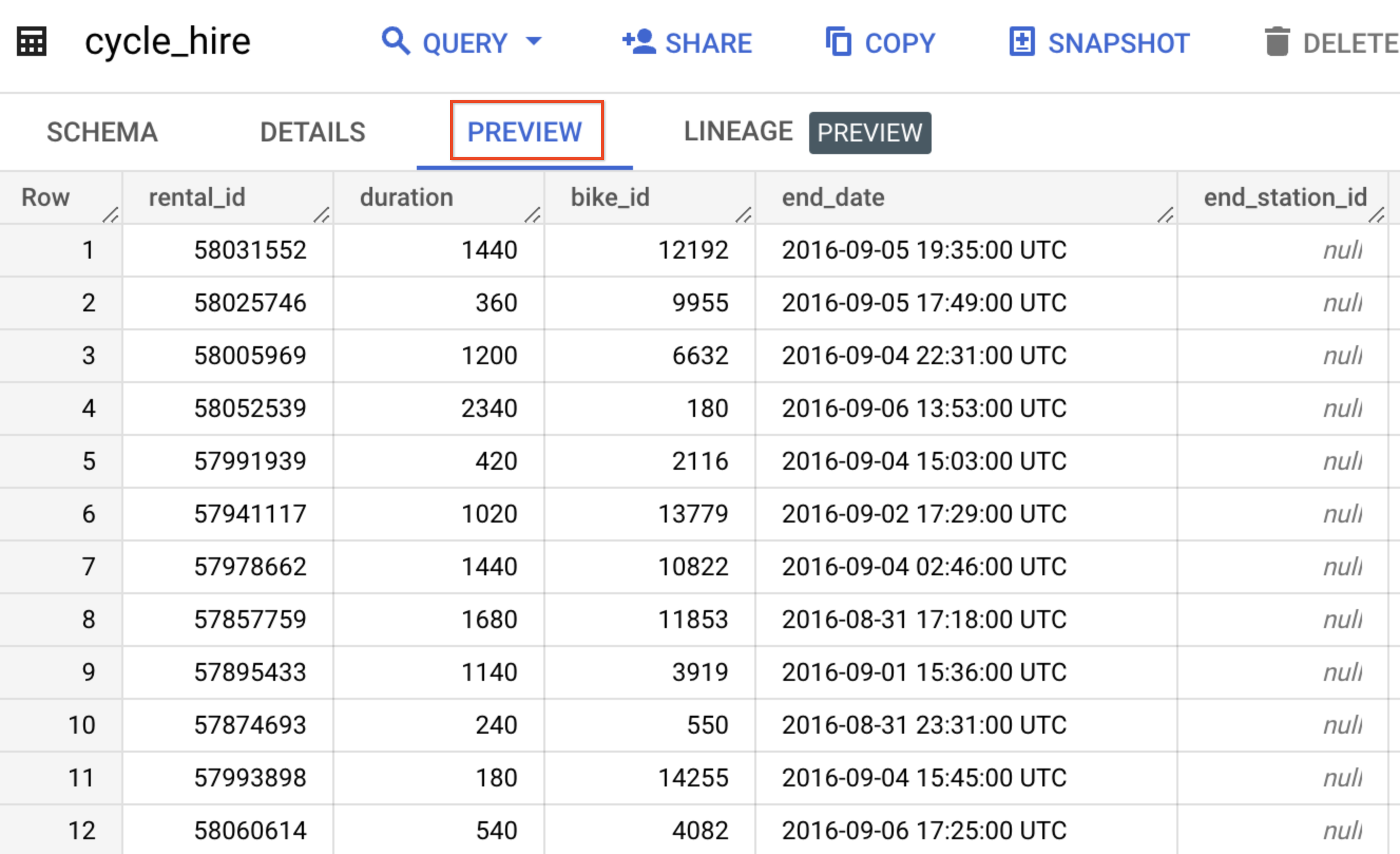
Inspect the columns and values populated in the rows. You are now ready to run some SQL queries on the cycle_hire table.

Running SELECT, FROM, and WHERE in BigQuery

You now have a basic understanding of SQL querying keywords and the BigQuery data paradigm and some data to work with. Run some SQL commands using this service.

If you look at the bottom right corner of the console, you will notice that there are 83,434,866 rows of data, or individual bikeshare trips taken in London between 2015 and 2017 (not a small amount by any means!)

Now take note of the seventh column key: end_station_name, which specifies the end destination of bikeshare rides. Before getting too deep, run a simple query to isolate the end_station_name column.

1. Copy and paste the following command into the query Editor:

SELECT end_station_name FROM `bigquery-public-data.london_bicycles.cycle_hire`;

2. Then click Run.

After ~20 seconds, you should be returned with 83434866 rows that contain the single column you queried for: end_station_name.

Why don't you find out how many bike trips were 20 minutes or longer?

3. Clear the query from the editor, then run the following query that utilizes the WHERE keyword:

SELECT * FROM `bigquery-public-data.london_bicycles.cycle_hire` WHERE duration>=1200;

This query may take a minute or so to run.

SELECT * returns all column values from the table. Duration is measured in seconds, which is why you used the value 1200 (60 * 20).

If you look in the bottom right corner you see that 26,441,016 rows were returned. As a fraction of the total (26441016/83434866), this means that ~30% of London bikeshare rides lasted 20 minutes or longer (they're in it for the long haul!)

Test your understanding

The following are some multiple choice questions to reinforce your understanding of the concepts we've covered so far. Answer them to the best of your abilities.

Task 3. More SQL Keywords: GROUP BY, COUNT, AS, and ORDER BY

GROUP BY

The GROUP BY keyword will aggregate result-set rows that share common criteria (e.g. a column value) and will return all of the unique entries found for such criteria.

This is a useful keyword for figuring out categorical information on tables.

1. To get a better picture of what this keyword does, clear the query from the editor, then copy and paste the following command:

SELECT start_station_name FROM `bigquery-public-data.london_bicycles.cycle_hire` GROUP BY start_station_name;

2. Click Run.

Your results are a list of unique (non-duplicate) column values.

Without the GROUP BY, the query would have returned the full 83,434,866 rows. GROUP BY will output the unique column values found in the table. You can see this for yourself by looking in the bottom right corner. You will see 954 rows, meaning there are 954 distinct London bikeshare starting points.

COUNT

The COUNT() function will return the number of rows that share the same criteria (e.g. column value). This can be very useful in tandem with a GROUP BY.

Add the COUNT function to our previous query to figure out how many rides begin at each starting point.

• Clear the query from the editor, then copy and paste the following command and then click Run:

SELECT start_station_name, COUNT(*) FROM `bigquery-public-data.london_bicycles.cycle_hire` GROUP BY start_station_name;

Your output shows how many bikeshare rides begin at each starting location.

AS

SQL also has an AS keyword, which creates an alias of a table or column. An alias is a new name that's given to the returned column or table—whatever AS specifies.

1. Add an AS keyword to the last query you ran to see this in action. Clear the query from the editor, then copy and paste the following command:

SELECT start_station_name, COUNT(*) AS num_starts FROM `bigquery-public-data.london_bicycles.cycle_hire` GROUP BY start_station_name;

2. Click Run.

For Results, the right column name changed from COUNT(*) to num_starts.

As you see, the COUNT(*) column in the returned table is now set to the alias name num_starts. This is a handy keyword to use especially if you are dealing with large sets of data — forgetting that an ambiguous table or column name happens more often than you think!

ORDER BY

The ORDER BY keyword sorts the returned data from a query in ascending or descending order based on a specified criteria or column value. Add this keyword to our previous query to do the following:

• Return a table that contains the number of bikeshare rides that begin at each starting station, organized alphabetically by the starting station.
• Return a table that contains the number of bikeshare rides that begin at each starting station, organized numerically from lowest to highest.
• Return a table that contains the number of bikeshare rides that begin at each starting station, organized numerically from highest to lowest.

Each of the commands below is a separate query. For each command:

1. Clear the query Editor.
2. Copy and paste the command into the query Editor.
3. Click Run. Examine the results.

SELECT start_station_name, COUNT(*) AS num FROM `bigquery-public-data.london_bicycles.cycle_hire` GROUP BY start_station_name ORDER BY start_station_name; SELECT start_station_name, COUNT(*) AS num FROM `bigquery-public-data.london_bicycles.cycle_hire` GROUP BY start_station_name ORDER BY num; SELECT start_station_name, COUNT(*) AS num FROM `bigquery-public-data.london_bicycles.cycle_hire` GROUP BY start_station_name ORDER BY num DESC;

The results of the last query lists start locations by the number of starts from that location.

You see that "Belgrove Street, King's Cross" has the highest number of starts. However, as a fraction of the total (234458/83434866), you see that < 1% of rides start from this station.

Test your understanding

The following are some multiple choice questions to reinforce your understanding of the concepts covered so far. Answer them to the best of your abilities.

Task 4. Working with Cloud SQL

Exporting queries as CSV files

Cloud SQL is a fully-managed database service that makes it easy to set up, maintain, manage, and administer your relational PostgreSQL and MySQL databases in the cloud. There are two formats of data accepted by Cloud SQL: dump files (.sql) or CSV files (.csv). You will learn how to export subsets of the cycle_hire table into CSV files and upload them to Cloud Storage as an intermediate location.

Back in the BigQuery Console, this should have been the last command that you ran:

SELECT start_station_name, COUNT(*) AS num FROM `bigquery-public-data.london_bicycles.cycle_hire` GROUP BY start_station_name ORDER BY num DESC;

1. In the Query Results section click SAVE RESULTS > CSV(local file). This initiates a download, which saves this query as a CSV file. Note the location and the name of this downloaded file—you will need it soon.

2. Clear the query Editor, then copy and run the following in the query editor:

SELECT end_station_name, COUNT(*) AS num FROM `bigquery-public-data.london_bicycles.cycle_hire` GROUP BY end_station_name ORDER BY num DESC;

This returns a table that contains the number of bikeshare rides that finish in each ending station and is organized numerically from highest to lowest number of rides.

3. In the Query Results section click SAVE RESULTS > CSV(local file). This initiates a download, which saves this query as a CSV file. Note the location and the name of this downloaded file—you will need it in the following section.

Upload CSV files to Cloud Storage

1. Go to the Cloud Console where you'll create a storage bucket where you can upload the files you just created.

2. Select Navigation menu > Cloud Storage > Buckets, and then click CREATE BUCKET.

Note: If prompted, click LEAVE for Unsaved work.

3. Enter a unique name for your bucket, keep all other settings as default, and click Create.

4. If prompted, click Confirm for Public access will be prevented dialog.

Test completed task

Click Check my progress below to check your lab progress. If you successfully created your bucket, you'll see an assessment score.

Create a cloud storage bucket.

You should now be in the Cloud Console looking at your newly created Cloud Storage Bucket.

1. Click UPLOAD FILES and select the CSV that contains start_station_name data.

2. Then click Open. Repeat this for the end_station_name data.

3. Rename your start_station_name file by clicking on the three dots next to on the far side of the file and click rename. Rename the file to start_station_data.csv.

4. Rename your end_station_name file by clicking on the three dots next to on the far side of the file and click rename. Rename the file to end_station_data.csv.

You should now see start_station_data.csv and end_station_data.csv in the Objects list on the Bucket details page.

Test completed task

Click Check my progress to verify your performed task. If you have successfully uploaded CSV objects to your bucket, you will see an assessment score.

Upload CSV files to Cloud Storage.

Task 5. Create a Cloud SQL instance

In the console, select Navigation menu > SQL.

1. Click CREATE INSTANCE > Choose MySQL .

2. Enter instance id as my-demo.

3. Enter a secure password in the Password field (remember it!).

4. Select the database version as MySQL 8.

5. For Choose a Cloud SQL edition, select Enterprise.

6. For Preset, select Development (4 vCPU, 16 GB RAM, 100 GB Storage, Single zone).

Warning: if you choose a preset larger than Development, your project will be flagged and your lab will be terminated.

7. Set the Multi zones (Highly available) field as

8. Click CREATE INSTANCE.

Note: It might take a few minutes for the instance to be created. Once it is, you will see a green checkmark next to the instance name on the SQL instances page.

9. Click on the Cloud SQL instance. The SQL Overview page opens.

Test completed task

To check out your lab progress, click Check my progress below. If you have successfully set up your Cloud SQL instance, you will see an assessment score.

Create a CloudSQL Instance.

Task 6. New queries in Cloud SQL

CREATE keyword (databases and tables)

Now that you have a Cloud SQL instance up and running, create a database inside of it using the Cloud Shell Command Line.

1. Open Cloud Shell by clicking on the icon in the top right corner of the console.

2. Run the following command to set your project ID as an environment variable:

export PROJECT_ID=$(gcloud config get-value project) gcloud config set project $PROJECT_ID

Create a database in Cloud Shell

1. Run the following command in Cloud Shell to setup auth without opening up a browser.

gcloud auth login --no-launch-browser

This will give you a link to open in your browser. Open the link in the same browser where you are logged in to the qwiklabs account. Once you login you will get a verification code to copy. Paste that code in the cloud shell.

2. Run the following command to connect to your SQL instance, replacing my-demo if you used a different name for your instance:

gcloud sql connect my-demo --user=root --quiet Note: It may take a minute to connect to your instance. If you get an message that "Operation failed because another operation was already in progress", you need to wait for the SQL instance to finish being created, and then try to connect again.

3. When prompted, enter the root password you set for the instance.

You should see similar output:

Welcome to the MySQL monitor. Commands end with ; or \g. Your MySQL connection id is 494 Server version: 8.0.31-google (Google) Copyright (c) 2000, 2017, Oracle, MariaDB Corporation Ab and others. Type 'help;' or '\h' for help. Type '\c' to clear the current input statement. mysql>

A Cloud SQL instance comes with pre-configured databases, but you will create your own to store the London bikeshare data.

4. Run the following command at the MySQL server prompt to create a database called bike:

CREATE DATABASE bike;

You should receive the following output:

Query OK, 1 row affected (0.05 sec) mysql>

Test completed task

Check your progress by clicking Check my progress to verify your performed task. If you have successfully created a database in the Cloud SQL instance, you will see an assessment score.

Create a database.

Create a table in Cloud Shell

1. Make a table inside of the bike database by running the following command:

USE bike; CREATE TABLE london1 (start_station_name VARCHAR(255), num INT);

This statement uses the CREATE keyword, but this time it uses the TABLE clause to specify that it wants to build a table instead of a database. The USE keyword specifies a database that you want to connect to. You now have a table named "london1" that contains two columns, "start_station_name" and "num". VARCHAR(255) specifies variable length string column that can hold up to 255 characters and INT is a column of type integer.

2. Create another table named "london2" by running the following command:

USE bike; CREATE TABLE london2 (end_station_name VARCHAR(255), num INT);

3. Now confirm that your empty tables were created. Run the following commands at the MySQL server prompt:

SELECT * FROM london1; SELECT * FROM london2;

You should receive the following output for both commands:

Empty set (0.04 sec)

You see "empty set" because you haven't yet loaded the data.

Upload CSV files to tables

Return to the Cloud SQL console. You will now upload the start_station_name and end_station_name CSV files into your newly created london1 and london2 tables.

1. In your Cloud SQL instance page, click IMPORT.
2. In the Cloud Storage file field, click Browse, and then click the arrow next to your bucket name, and then click start_station_data.csv. Click Select.
3. Select CSV as File format.
4. Select the bike database and type in london1 as your table.
5. Click Import.

Do the same for the other CSV file.

1. In your Cloud SQL instance page, click IMPORT.
2. In the Cloud Storage file field, click Browse, and then click the arrow next to your bucket name, and then click end_station_data.csv Click Select.
3. Select CSV as File format.
4. Select the bike database and type in london2 as your table.
5. Click Import.

You should now have both CSV files uploaded to tables in the bike database.

1. Return to your Cloud Shell session and run the following command at the MySQL server prompt to inspect the contents of london1:

SELECT * FROM london1;

You should receive 955 lines of output, one for each unique station name.

2. Run the following command to make sure that london2 has been populated:

SELECT * FROM london2;

You should receive 959 lines of output, one more each unique station name.

DELETE keyword

Here are a couple more SQL keywords that help us with data management. The first is the DELETE keyword.

• Run the following commands in your MySQL session to delete the first row of the london1 and london2:

DELETE FROM london1 WHERE num=0; DELETE FROM london2 WHERE num=0;

You should receive the following output after running both commands:

Query OK, 1 row affected (0.04 sec)

The rows deleted were the column headers from the CSV files. The DELETE keyword will not remove the first row of the file per se, but all rows of the table where the column name (in this case "num") contains a specified value (in this case "0"). If you run the SELECT * FROM london1; and SELECT * FROM london2; queries and scroll to the top of the table, you will see that those rows no longer exist.

INSERT INTO keyword

You can also insert values into tables with the INSERT INTO keyword.

• Run the following command to insert a new row into london1, which sets start_station_name to "test destination" and num to "1":

INSERT INTO london1 (start_station_name, num) VALUES ("test destination", 1);

The INSERT INTO keyword requires a table (london1) and will create a new row with columns specified by the terms in the first parenthesis (in this case "start_station_name" and "num"). Whatever comes after the "VALUES" clause will be inserted as values in the new row.

You should receive the following output:

Query OK, 1 row affected (0.05 sec)

If you run the query SELECT * FROM london1; you will see an additional row added at the bottom of the "london1" table.

UNION keyword

The last SQL keyword that you'll learn about is UNION. This keyword combines the output of two or more SELECT queries into a result-set. You use UNION to combine subsets of the "london1" and "london2" tables.

The following chained query pulls specific data from both tables and combines them with the UNION operator.

• Run the following command at the MySQL server prompt:

SELECT start_station_name AS top_stations, num FROM london1 WHERE num>100000 UNION SELECT end_station_name, num FROM london2 WHERE num>100000 ORDER BY top_stations DESC;

The first SELECT query selects the two columns from the "london1" table and creates an alias for "start_station_name", which gets set to "top_stations". It uses the WHERE keyword to only pull rideshare station names where over 100,000 bikes start their journey.

The second SELECT query selects the two columns from the "london2" table and uses the WHERE keyword to only pull rideshare station names where over 100,000 bikes end their journey.

The UNION keyword in between combines the output of these queries by assimilating the "london2" data with "london1". Since "london1" is being unioned with "london2", the column values that take precedence are "top_stations" and "num".

ORDER BY will order the final, unioned table by the "top_stations" column value alphabetically and in descending order.

You should receive the following output:

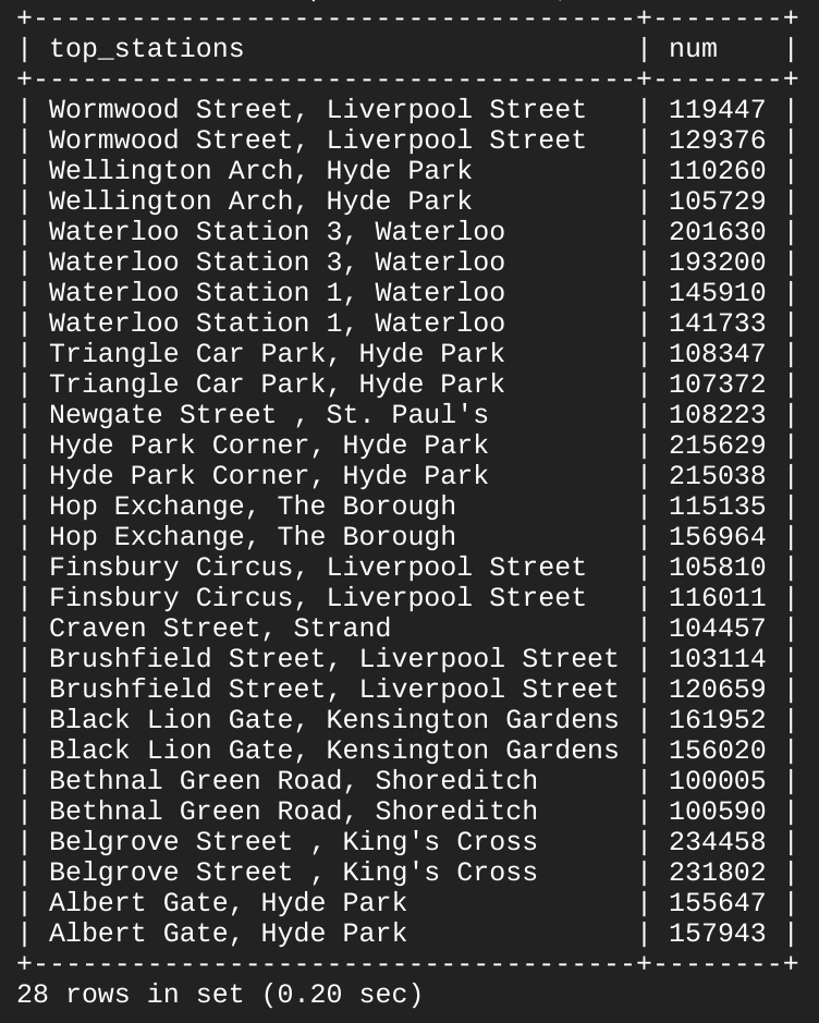
As you see, 13/14 stations share the top spots for rideshare starting and ending points. With some basic SQL keywords you were able to query a sizable dataset, which returned data points and answers to specific questions.

Congratulations!

In this lab, you learned the fundamentals of SQL and how you can apply keywords and run queries in BigQuery and CloudSQL. You were taught the core concepts behind projects, databases, and tables. You practiced with keywords that manipulated and edited data. You learned how to read data into BigQuery and you practiced running queries on tables. You learned how to create instances in Cloud SQL and practiced transferring subsets of data into tables contained in databases. You chained and ran queries in Cloud SQL to arrive at some interesting conclusions about London bikesharing starting and ending stations.

Next steps / Learn more

Continue to learn and practice with Cloud SQL and BigQuery with these Google Cloud Skill Boost labs:

• Weather Data in BigQuery
• Exploring NCAA Data with BigQuery
• Loading Data into Google Cloud SQL
• Cloud SQL with Terraform

Learn more about Data Science with Data Science on the Google Cloud Platform, 2nd Edition: O'Reilly Media, Inc..

Google Cloud training and certification

...helps you make the most of Google Cloud technologies. Our classes include technical skills and best practices to help you get up to speed quickly and continue your learning journey. We offer fundamental to advanced level training, with on-demand, live, and virtual options to suit your busy schedule. Certifications help you validate and prove your skill and expertise in Google Cloud technologies.

Manual Last Updated February 02, 2024

Lab Last Tested February 02, 2024

Copyright 2024 Google LLC All rights reserved. Google and the Google logo are trademarks of Google LLC. All other company and product names may be trademarks of the respective companies with which they are associated.