GSP271

Overview

Introduction

In this lab you implement logistic regression using a machine learning library for Apache Spark. Spark runs on a Dataproc cluster to develop a model for data from a multivariable dataset.

Dataproc is a fast, easy-to-use, fully-managed cloud service for running Apache Spark and Apache Hadoop clusters in a simple, cost-efficient way. Dataproc easily integrates with other Google Cloud services, giving you a powerful and complete platform for data processing, analytics and machine learning

Apache Spark is an analytics engine for large scale data processing. Logistic regression is available as a module in Apache Spark's machine learning library, MLlib. Spark MLlib, also called Spark ML, includes implementations for most standard machine learning algorithms such as k-means clustering, random forests, alternating least squares, k-means clustering, decision trees, support vector machines, etc. Spark can run on a Hadoop cluster, like Dataproc, in order to process very large datasets in parallel.

The base dataset this lab uses is retrieved from the US Bureau of Transport Statistics. The dataset provides historical information about internal flights in the United States and can be used to demonstrate a wide range of data science concepts and techniques. This lab provides the data as a set of CSV formatted text files.

Objectives

• Create a training dataset for machine learning using Spark
• Develop a logistic regression machine learning model using Spark
• Evaluate the predictive behavior of a machine learning model using Spark on Dataproc
• Evaluate the model

Setup and requirements

Before you click the Start Lab button

Read these instructions. Labs are timed and you cannot pause them. The timer, which starts when you click Start Lab, shows how long Google Cloud resources will be made available to you.

This hands-on lab lets you do the lab activities yourself in a real cloud environment, not in a simulation or demo environment. It does so by giving you new, temporary credentials that you use to sign in and access Google Cloud for the duration of the lab.

To complete this lab, you need:

• Access to a standard internet browser (Chrome browser recommended).

Note: Use an Incognito or private browser window to run this lab. This prevents any conflicts between your personal account and the Student account, which may cause extra charges incurred to your personal account.

• Time to complete the lab---remember, once you start, you cannot pause a lab.

Note: If you already have your own personal Google Cloud account or project, do not use it for this lab to avoid extra charges to your account.

How to start your lab and sign in to the Google Cloud console

1. Click the Start Lab button. If you need to pay for the lab, a pop-up opens for you to select your payment method. On the left is the Lab Details panel with the following:

   • The Open Google Cloud console button
   • Time remaining
   • The temporary credentials that you must use for this lab
   • Other information, if needed, to step through this lab

2. Click Open Google Cloud console (or right-click and select Open Link in Incognito Window if you are running the Chrome browser).

   The lab spins up resources, and then opens another tab that shows the Sign in page.

   Tip: Arrange the tabs in separate windows, side-by-side.

   Note: If you see the Choose an account dialog, click Use Another Account.

3. If necessary, copy the Username below and paste it into the Sign in dialog.

   {{{user_0.username | "Username"}}}

   You can also find the Username in the Lab Details panel.

4. Click Next.

5. Copy the Password below and paste it into the Welcome dialog.

   {{{user_0.password | "Password"}}}

   You can also find the Password in the Lab Details panel.

6. Click Next.

   Important: You must use the credentials the lab provides you. Do not use your Google Cloud account credentials. Note: Using your own Google Cloud account for this lab may incur extra charges.

7. Click through the subsequent pages:

   • Accept the terms and conditions.
   • Do not add recovery options or two-factor authentication (because this is a temporary account).
   • Do not sign up for free trials.

After a few moments, the Google Cloud console opens in this tab.

Note: To view a menu with a list of Google Cloud products and services, click the Navigation menu at the top-left.

Task 1. Create a Dataproc cluster

Normally, the first step in writing Hadoop jobs is to get a Hadoop installation going. This involves setting up a cluster, installing Hadoop on it, and configuring the cluster so that the machines all know about one another and can communicate with one another in a secure manner.

Then, you’d start the YARN and MapReduce processes and finally be ready to write some Hadoop programs. On Google Cloud, Dataproc makes it convenient to spin up a Hadoop cluster that is capable of running MapReduce, Pig, Hive, Presto, and Spark.

If you are using Spark, Dataproc offers a fully managed, serverless Spark environment – you simply submit a Spark program and Dataproc executes it. In this way, Dataproc is to Apache Spark what Dataflow is to Apache Beam. In fact, Dataproc and Dataflow share backend services.

In this section you create a VM and then a Dataproc cluster on the VM.

1. In the Cloud Console, on the Navigation menu (), click Compute Engine > VM instances.

2. Click the SSH button next to startup-vm VM to launch a terminal and connect.

3. Click Connect to confirm the SSH connection.

4. Run following command to clone the repository data-science-on-gcp, and navigate to the directory 06_dataproc:

git clone https://github.com/GoogleCloudPlatform/data-science-on-gcp/ cd ~/data-science-on-gcp/06_dataproc

5. Set the project and bucket variable using the following code:

export PROJECT_ID=$(gcloud info --format='value(config.project)') export BUCKET_NAME=$PROJECT_ID-dsongcp

6. Edit the create_cluster.sh file by removing the zonal dependency code --zone ${REGION}-a

nano create_cluster.sh

Your output should similar to the following:

gcloud dataproc clusters create ch6cluster \ --enable-component-gateway \ --region ${REGION} \ --master-machine-type n1-standard-4 \ --master-boot-disk-size 500 --num-workers 2 \ --worker-machine-type n1-standard-4 \ --worker-boot-disk-size 500 \ --optional-components JUPYTER --project $PROJECT \ --initialization-actions=$INSTALL \ --scopes https://www.googleapis.com/auth/cloud-platform

7. Save file by using Ctrl+X press Y and enter

8. Create a Dataproc cluster to run jobs on, specifying the name of your bucket and the region that the bucket is in:

./create_cluster.sh $BUCKET_NAME {{{ project_0.default_region | "REGION" }}}

This command may take a few minutes.

Note: When performing these tasks outside of this lab, the compute zone must be in the same region as the bucket to avoid network egress charges. Create Cloud Dataproc cluster

JupyterLab on Dataproc

1. In the Cloud Console, on the Navigation menu, click Dataproc. You may have to click More Products and scroll down.

2. In the Cluster list, click on the cluster name to view cluster details.

3. Click the Web Interfaces tab and then click JupyterLab towards the bottom of the right pane.

4. In the Notebook launcher section click Python 3 to open a new notebook.

To use a Notebook you enter commands into a cell. Be sure you run the commands in the cell by either pressing Shift + Enter, or clicking the triangle on the Notebook top menu to Run selected cells and advance.

Task 2. Set up bucket and start pyspark session

1. Set up a google cloud storage bucket where your raw files are hosted:

PROJECT=!gcloud config get-value project PROJECT=PROJECT[0] BUCKET = PROJECT + '-dsongcp' import os os.environ['BUCKET'] = PROJECT + '-dsongcp'

2. Run the cell by either pressing Shift + Enter, or clicking the triangle on the Notebook top menu to Run selected cells and advance.

Note: After pasting commands into the Jupyter notebook cell, always run the cell to execute the command and advance to the next cell.

3. Create a spark session using the following code block:

from pyspark.sql import SparkSession from pyspark import SparkContext sc = SparkContext('local', 'logistic') spark = SparkSession \ .builder \ .appName("Logistic regression w/ Spark ML") \ .getOrCreate()

Once that code is added at the start of any Spark Python script, any code developed using the interactive Spark shell or Jupyter notebook will also work when launched as a standalone script.

Create a Spark Dataframe for training

1. Enter the following commands into new cell:

from pyspark.mllib.classification import LogisticRegressionWithLBFGS from pyspark.mllib.regression import LabeledPoint

2. Run the cell.

Note: When pasting commands into the Jupyter notebook cell remember to run the cell to make sure that the last command in any sequence is executed before you proceed to the next step.

Task 3. Read and clean up dataset

When you launched this lab, an automated script provided data to you as a set of prepared CSV files and was placed into your Cloud Storage bucket.

• Now, fetch the Cloud Storage bucket name from the environment variable you set earlier and create the traindays DataFrame by reading in a prepared CSV that the automated script puts into your Cloud Storage bucket.

The CSV identifies a subset of days as valid for training. This allows you to create views of the entire flights dataset which is divided into a dataset used for training your model and a dataset used to test or validate that model.

Read the dataset

1. Enter and run the following commands into the new cell:

traindays = spark.read \ .option("header", "true") \ .csv('gs://{}/flights/trainday.csv'.format(BUCKET)) traindays.createOrReplaceTempView('traindays')

2. Create a Spark SQL view:

traindays.createOrReplaceTempView('traindays')

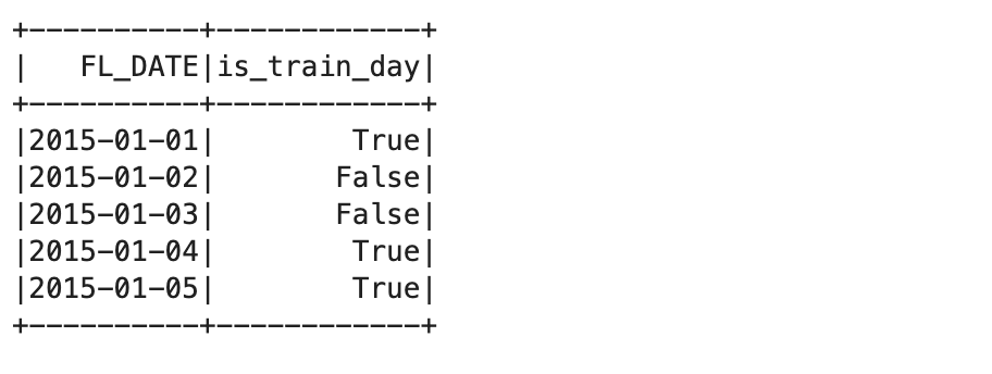
3. Query the first few records from the training dataset view:

spark.sql("SELECT * from traindays LIMIT 5").show()

This displays the first five records in the training table:

The next stage in the process is to identify the source data files.

4. You will use the all_flights-00000-* shard file for this, as it has a representative subset of the full dataset and can be processed in a reasonable amount of time:

inputs = 'gs://{}/flights/tzcorr/all_flights-00000-*'.format(BUCKET) Note: To process the full dataset, change the previous line to the following: #inputs = 'gs://{}/flights/tzcorr/all_flights-*'.format(BUCKET) # FULL

5. Now read the data into Spark SQL from the input file you created:

flights = spark.read.json(inputs) flights.createOrReplaceTempView('flights')

6. Next, create a query that uses data only from days identified as part of the training dataset:

trainquery = """ SELECT DEP_DELAY, TAXI_OUT, ARR_DELAY, DISTANCE FROM flights f JOIN traindays t ON f.FL_DATE == t.FL_DATE WHERE t.is_train_day == 'True' """ traindata = spark.sql(trainquery)

7. Inspect some of the data to see if it looks correct:

print(traindata.head(2)) Note: You may see a warning stating "Truncated the string representation of a plan since it was too large." For this lab, ignore it as it's only relevant if you want to inspect SQL schema logs.

Your output should be something similar to the following:

[Row(DEP_DELAY=-2.0, TAXI_OUT=26.0, ARR_DELAY=0.0, DISTANCE=677.0), Row(DEP_DELAY=-2.0, TAXI_OUT=22.0, ARR_DELAY=3. 0, DISTANCE=451.0)]

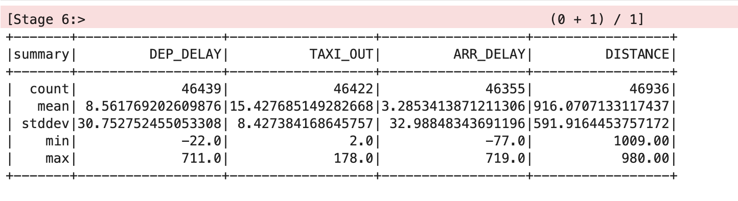
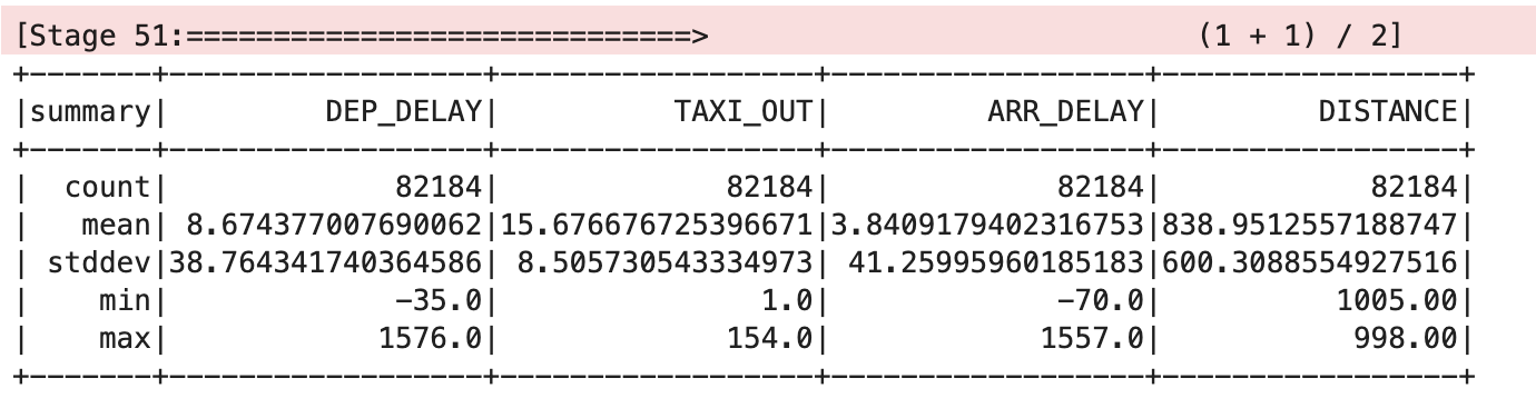
8. Ask Spark to provide some analysis of the dataset:

traindata.describe().show()

This should output something similar to the following:

Clean the dataset

The mean and standard deviation values have been rounded to two decimal places for clarity in this table, but you will see the full floating point values on screen.

The table shows that there are some issues with the data. Not all of the records have values for all of the variables, there are different count stats for DEP_DELAY, TAXI_OUT, ARR_DELAY and DISTANCE. This happens because:

• Flights are scheduled but never depart
• Some depart but are cancelled before take off
• Some flights are diverted and therefore never arrive

Note: The counts for the various columns are all different; we have to remove NULLs in the delay variables (these correspond to canceled or diverted flights).

1. Enter following code in new cell: trainquery = """ SELECT DEP_DELAY, TAXI_OUT, ARR_DELAY, DISTANCE FROM flights f JOIN traindays t ON f.FL_DATE == t.FL_DATE WHERE t.is_train_day == 'True' AND f.dep_delay IS NOT NULL AND f.arr_delay IS NOT NULL """ traindata = spark.sql(trainquery) traindata.describe().show()

This should output something similar to the following:

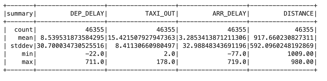
2. Remove flights that have been cancelled or diverted using the following query:

trainquery = """ SELECT DEP_DELAY, TAXI_OUT, ARR_DELAY, DISTANCE FROM flights f JOIN traindays t ON f.FL_DATE == t.FL_DATE WHERE t.is_train_day == 'True' AND f.CANCELLED == 'False' AND f.DIVERTED == 'False' """ traindata = spark.sql(trainquery) traindata.describe().show()

This output should show the same count value for each column, which indicates that you fixed the problem.

Task 4. Develop a logistic regression model

Now you can create a function that converts a set of data points in your DataFrame into a training example. A training example contains a sample of the input features and the correct answer for those inputs.

In this case, you answer whether the arrival delay is less than 15 minutes. The labels you use as inputs are the values for departure delay, taxi out time, and flight distance.

1. Enter and run the following into the new cell to create the definition for the training example function:

def to_example(fields): return LabeledPoint(\ float(fields['ARR_DELAY'] < 15), #ontime? \ [ \ fields['DEP_DELAY'], \ fields['TAXI_OUT'], \ fields['DISTANCE'], \ ])

2. Map this training example function to the training dataset:

examples = traindata.rdd.map(to_example)

3. Enter and run the following command to provide a training DataFrame for the Spark logistic regression module:

lrmodel = LogisticRegressionWithLBFGS.train(examples, intercept=True)

The training DataFrame creates a logistic regression model based on your training dataset.

• Use the intercept=True parameter because the prediction for arrival delay does not equal zero when all of the inputs are zero in this case.
• If you have a training dataset where you expect that a prediction should be zero when the inputs are all zero, then you would specify intercept=False.

4. When this train method finishes, the lrmodel object will have weights and an intercept value that you can inspect:

print(lrmodel.weights,lrmodel.intercept)

The output looks similar to the following:

[-0.17926510230641074,-0.1353410840270897,0.00047781052266304745] 5.403405250989946

These weights, when used with the formula for linear regression, allow you to create a model using code in the language of your choice.

5. Test this by providing some input variables for a flight that has:

• A departure delay of 6 minutes
• A taxi-out time of 12 minutes
• A flight distance of 594 miles

print(lrmodel.predict([6.0,12.0,594.0]))

The result of 1 predicts the flight will be on time.

6. Now try it with a much longer departure delay of 36 minutes:

print(lrmodel.predict([36.0,12.0,594.0]))

The result of 0 predicts the flight won't be on time.

These results are not probabilities; they are returned as either true or false based on a threshold which is set by default to 0.5.

7. You can return the actual probability by clearing the threshold:

lrmodel.clearThreshold() print(lrmodel.predict([6.0,12.0,594.0])) print(lrmodel.predict([36.0,12.0,594.0]))

Notice the results are probabilities, with the first close to 1 and the second close to 0.

8. Set the threshold to 0.7 to correspond to your requirement to be able to cancel meetings if the probability of an on time arrival falls below 70%:

lrmodel.setThreshold(0.7) print(lrmodel.predict([6.0,12.0,594.0])) print(lrmodel.predict([36.0,12.0,594.0]))

Your outputs are once again 1 and 0, but now they reflect the 70% probability threshold that you require and not the default 50%.

Task 5. Save and restore a logistic regression model

You can save a Spark logistic regression model directly to Cloud Storage. This allows you to reuse a model without having to retrain the model from scratch.

A storage location contains only one model. This avoids interference with other existing files which would cause model loading issues. To do this, make sure your storage location is empty before you save your Spark regression model.

1. Enter the following code in new cell and run:

MODEL_FILE='gs://' + BUCKET + '/flights/sparkmloutput/model' os.system('gsutil -m rm -r ' + MODEL_FILE)

This should report an error stating CommandException: 1 files/objects could not be removed because the model has not been saved yet. The error indicates that there are no files present in the target location. You must be certain that this location is empty before attempting to save the model and this command guarantees that.

2. Save the model by running:

lrmodel.save(sc, MODEL_FILE) print('{} saved'.format(MODEL_FILE))

3. Now destroy the model object in memory and confirm that it no longer contains any model data:

lrmodel = 0 print(lrmodel)

4. Now retrieve the model from storage:

from pyspark.mllib.classification import LogisticRegressionModel lrmodel = LogisticRegressionModel.load(sc, MODEL_FILE) lrmodel.setThreshold(0.7)

The model parameters, i.e. the weights and intercept values, have been restored.

Create a logistic regression model

Task 6. Predict with the logistic regression model

1. Test the model with a scenario that will definitely not arrive on time:

print(lrmodel.predict([36.0,12.0,594.0]))

This prints out 0, predicting the flight will probably arrive late, given your 70% probability threshold.

2. Finally, retest the model using data for a flight that should arrive on time:

print(lrmodel.predict([8.0,4.0,594.0]))

This prints out 1, predicting that the flight will probably arrive on time, given your 70% probability threshold.

Task 7. Examine model behavior

1. Enter the following code into a new cell and run the cell:

lrmodel.clearThreshold() # to make the model produce probabilities print(lrmodel.predict([20, 10, 500]))

With the thresholds removed, you get probabilities. The probability of arriving late increases as the departure delay increases.

2. At a departure delay of 20 minutes and a taxi-out time of 10 minutes, this is how the distance affects the probability that the flight is on time:

import matplotlib.pyplot as plt import seaborn as sns import pandas as pd import numpy as np dist = np.arange(10, 2000, 10) prob = [lrmodel.predict([20, 10, d]) for d in dist] sns.set_style("whitegrid") ax = plt.plot(dist, prob) plt.xlabel('distance (miles)') plt.ylabel('probability of ontime arrival')

As you can see, the effect is relatively minor. The probability increases from about 0.63 to about 0.76 as the distance changes from a very short hop to a cross-continent flight.

3. Run the following in new cell:

delay = np.arange(-20, 60, 1) prob = [lrmodel.predict([d, 10, 500]) for d in delay] ax = plt.plot(delay, prob) plt.xlabel('departure delay (minutes)') plt.ylabel('probability of ontime arrival')

On the other hand, if you hold the taxi-out time and distance constant and examine the dependence on departure delay, you see a more dramatic impact.

Task 8. Evaluate the model

1. To evaluate the logistic regression model, you need test data:

inputs = 'gs://{}/flights/tzcorr/all_flights-00001-*'.format(BUCKET) flights = spark.read.json(inputs) flights.createOrReplaceTempView('flights') testquery = trainquery.replace("t.is_train_day == 'True'","t.is_train_day == 'False'")

2. Now map this training example function to the testing dataset:

testdata = spark.sql(testquery) examples = testdata.rdd.map(to_example)

3. Ask Spark to provide some analysis of the dataset:

testdata.describe().show()

This should output something similar to the following:

4. Define a eval function and return total cancel, total noncancel, correct cancel and correct noncancel flight details:

def eval(labelpred): ''' data = (label, pred) data[0] = label data[1] = pred ''' cancel = labelpred.filter(lambda data: data[1] < 0.7) nocancel = labelpred.filter(lambda data: data[1] >= 0.7) corr_cancel = cancel.filter(lambda data: data[0] == int(data[1] >= 0.7)).count() corr_nocancel = nocancel.filter(lambda data: data[0] == int(data[1] >= 0.7)).count() cancel_denom = cancel.count() nocancel_denom = nocancel.count() if cancel_denom == 0: cancel_denom = 1 if nocancel_denom == 0: nocancel_denom = 1 return {'total_cancel': cancel.count(), \ 'correct_cancel': float(corr_cancel)/cancel_denom, \ 'total_noncancel': nocancel.count(), \ 'correct_noncancel': float(corr_nocancel)/nocancel_denom \ }

5. Now, evaluate the model by passing correct predicted label:

lrmodel.clearThreshold() # so it returns probabilities labelpred = examples.map(lambda p: (p.label, lrmodel.predict(p.features))) print('All flights:') print(eval(labelpred))

Output:

All flights: {'total_cancel': 14689, 'correct_cancel': 0.8239498944788617, 'total_noncancel': 67495, 'correct_noncancel': 0.9556411586043411}

6. Keep only those examples near the decision threshold which is greater than 65% and less than 75%:

print('Flights near decision threshold:') labelpred = labelpred.filter(lambda data: data[1] > 0.65 and data[1] < 0.75) print(eval(labelpred))

Output:

Flights near decision threshold: {'total_cancel': 714, 'correct_cancel': 0.3711484593837535, 'total_noncancel': 850, 'correct_noncancel': 0.6788235294117647}

Congratulations!

Now you know how to use Spark to perform logistic regression with a Dataproc cluster.

Take your next lab

Continue with:

• Machine Learning with TensorFlow in Vertex AI

Next steps / learn more

• Data Science on the Google Cloud Platform, 2nd Edition: O'Reilly Media, Inc.

Google Cloud training and certification

...helps you make the most of Google Cloud technologies. Our classes include technical skills and best practices to help you get up to speed quickly and continue your learning journey. We offer fundamental to advanced level training, with on-demand, live, and virtual options to suit your busy schedule. Certifications help you validate and prove your skill and expertise in Google Cloud technologies.

Manual Last Updated December 04, 2023

Lab Last Tested December 04, 2023

Copyright 2024 Google LLC All rights reserved. Google and the Google logo are trademarks of Google LLC. All other company and product names may be trademarks of the respective companies with which they are associated.